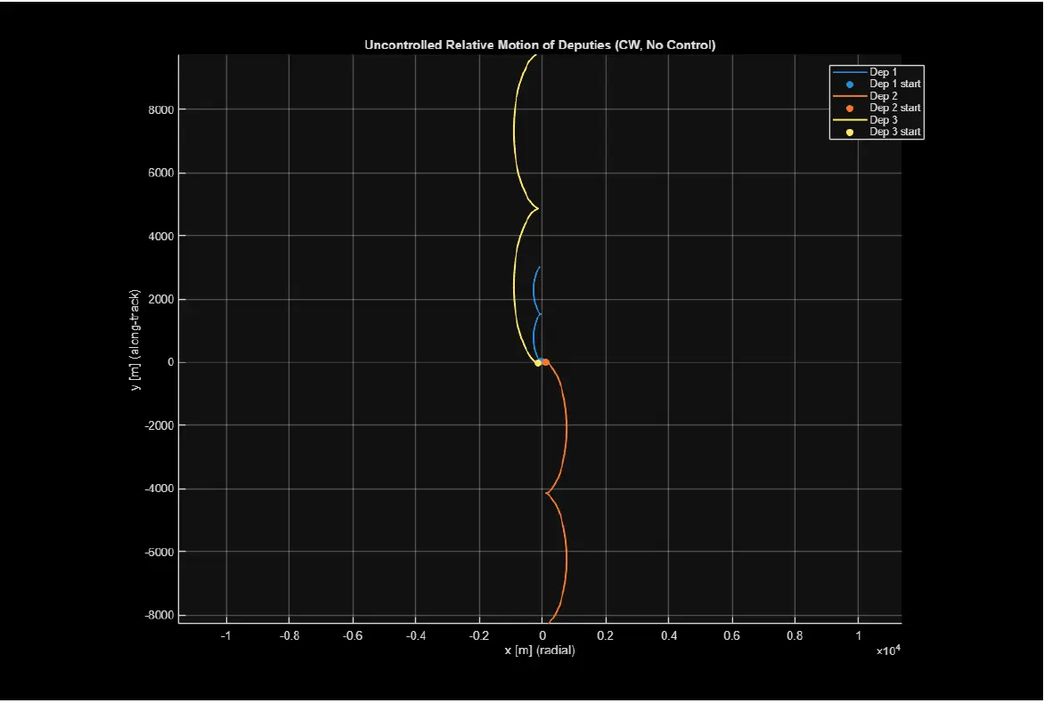
Three deputy spacecraft must hold fixed LVLH offsets while natural CW coupling and small acceleration disturbances drive uncontrolled drift.
Orbital DynamicsGuidance & ControlUSC Graduate Controls Project
Project 01 / GNC
Formation Control of Multiple Satellites in Orbit
A MATLAB trade study of how three deputy spacecraft can hold a commanded formation around a chief spacecraft—despite coupled orbital dynamics, limited thrust, and stochastic acceleration disturbances.
500 kmReference LEO altitude
20 sController sample time
3 hSimulation horizon
3Controllers compared
01 / Mission
Hold the formation without overpowering the physics.
Formation flying enables distributed sensing and cooperative space missions, but a deputy does not remain fixed simply because its initial position is close to the target. Radial and along-track motion are coupled, while cross-track motion oscillates.
The study commands three fixed LVLH positions—(0, 50, 0), (50, −50, 0), and (−50, −50, 0) meters—and evaluates control strategies using matched initial conditions and a common dynamics model.
02 / Engineering challenge + impact
The project in STAR form.
Build one repeatable MATLAB environment and compare stabilizing performance, thrust discipline, robustness, and computational tradeoffs.
Selected the CW/Hill model, discretized it at 20 seconds, implemented and tuned LQR and two MPC strategies, then generated matched trajectory and error plots.
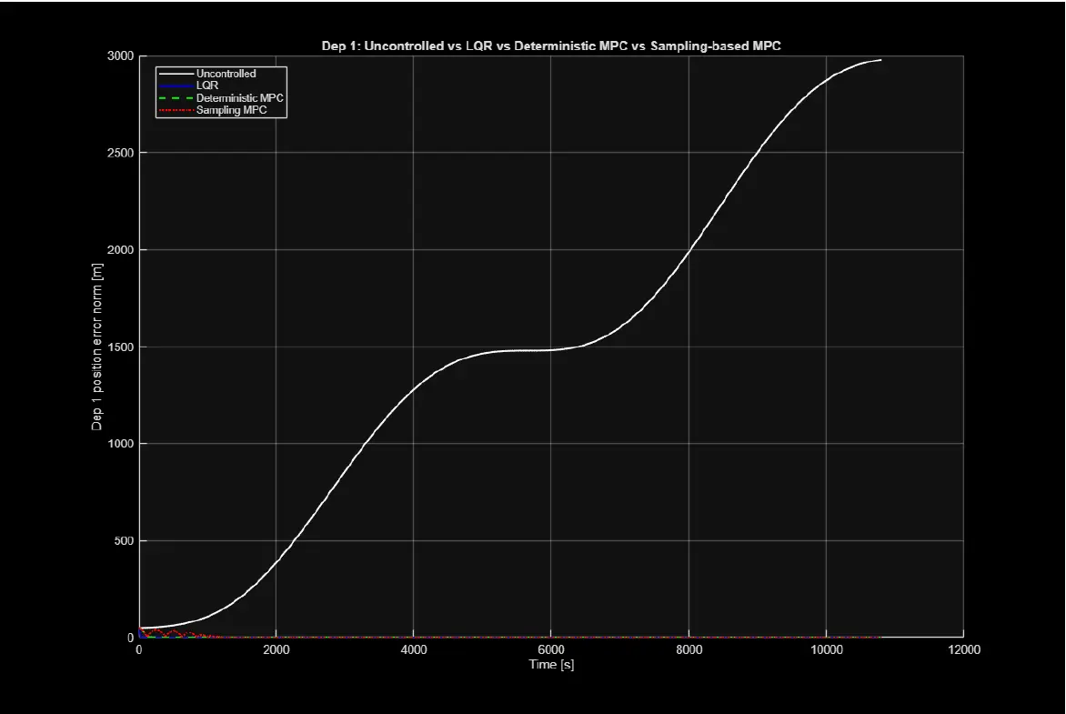
Every controller arrested the kilometer-scale uncontrolled divergence; LQR converged most directly, D-MPC enforced bounds, and sampled MPC improved disturbance awareness at greater cost.
My contribution
Model, implement, tune.
I selected the relative-motion model, built the final MATLAB simulation, implemented and tuned the controllers, and generated the performance plots. An early Python version served as a prototype before the final MATLAB implementation.
Two-person engineering project. This case study focuses only on my technical contribution and the shared project results.
03 / Dynamic model
Clohessy–Wiltshire relative motion
The chief follows a circular reference orbit. Each deputy uses a six-state LVLH representation, discretized with zero-order hold for the controller implementation.
ẍ − 2nẏ − 3n²x = uₓÿ + 2nẋ = uᵧz̈ + n²z = uᶻX = [x y z ẋ ẏ ż]ᵀ
xₖ₊₁ = Aᵈxₖ + Bᵈ(uₖ + wₖ)
‖uₖ‖∞ ≤ 5×10⁻³ m/s²
500 km circular LEO · Tₛ = 20 s · Tᶠ = 3 h
04 / Controller design
Shared objective. Different decision logic.
All three strategies use the same state and control weighting. Position error carries ten times the weight of velocity error, while the identity input penalty discourages excessive acceleration.
Controller weightsQ = diag(1, 1, 1, 0.1, 0.1, 0.1)R = I₃Position · velocity · control effort
Quadratic objectiveJ = Σ[(xₖ − xᵣ)ᵀQ(xₖ − xᵣ) + uₖᵀRuₖ]
Infinite-horizon feedback
MATLAB dlqr computes K for uₖ = −K(xₖ − xᵣ). The implemented disturbance study uses σ = 2×10⁻⁴ m/s².
Constrained receding horizon
A 10-step QP is solved with quadprog; only the first input is applied. A saturated LQR action is retained as a solver fallback.
Sampled expected cost
One LQR baseline plus 40 jittered candidates are each evaluated over 3 disturbance samples. Prediction and plant noise use σ = 4×10⁻⁵ m/s².
05 / Controller-specific results
Uncontrolled drift versus active formation keeping.
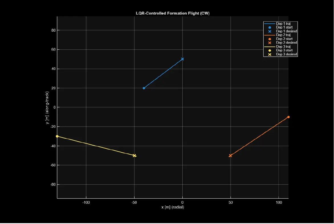
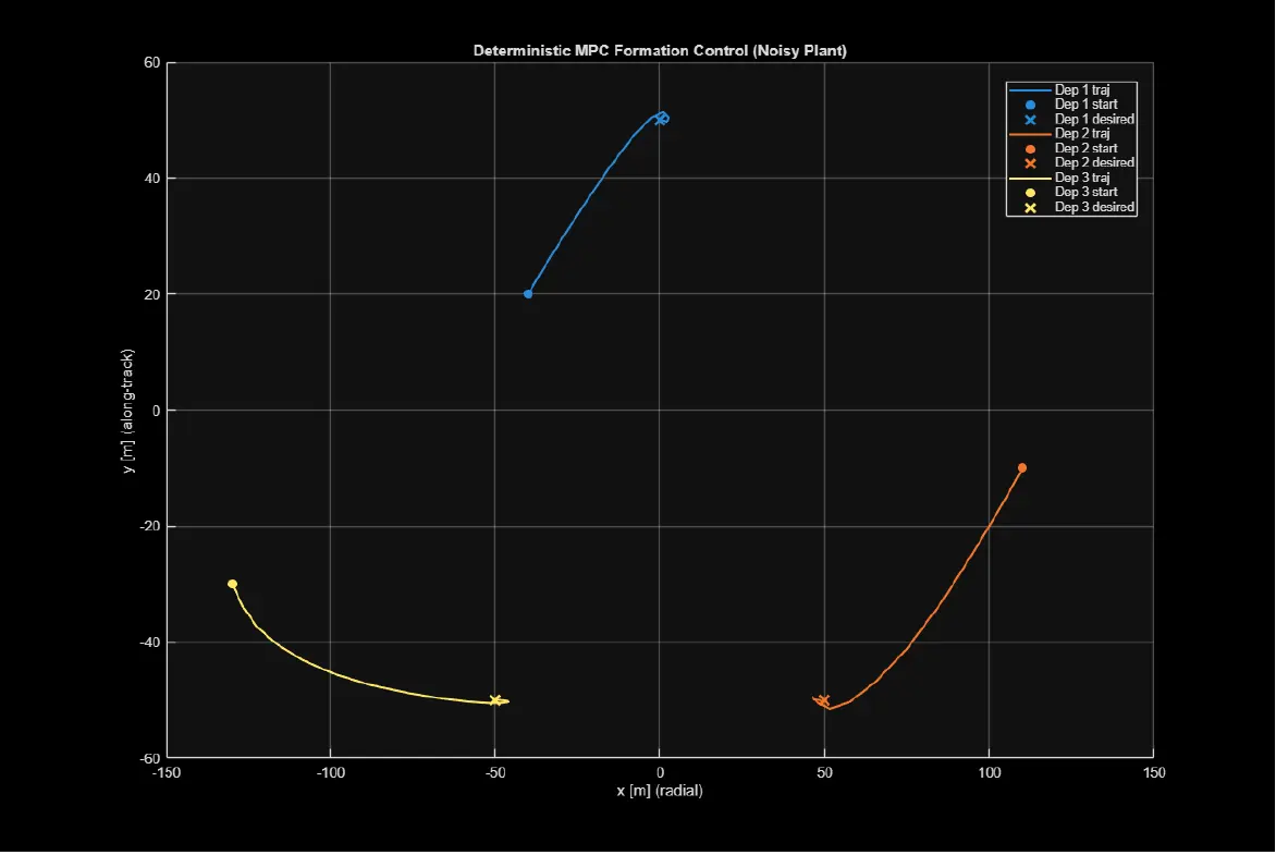
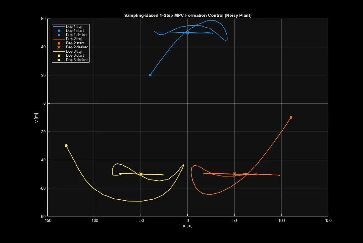
The plots below come directly from the final MATLAB implementation. Scale is the clearest result: the uncontrolled solution expands to kilometers, while the controlled cases remain concentrated around meter-scale formation targets.
01
Uncontrolled baseline
With u = 0, the same initial offsets grow into kilometer-scale along-track drift over the three-hour run. This establishes the failure mode each controller must suppress.
02
LQR
The discrete feedback law drives each deputy directly toward its commanded point. Relative to the baseline, the motion remains localized and convergence is computationally inexpensive.
03
Deterministic MPC
The receding-horizon QP bends trajectories smoothly into the formation while applying the modeled thrust limits. Its nominal prediction is less disturbance-aware than the sampled controller.
04
Sampling-based MPC
Candidate actions are tested against multiple disturbance draws. The resulting paths are more circuitous, but the controller explicitly selects for expected performance under uncertainty.
06 / Controller trade study
No universal winner—only the right tradeoff.
ControllerStrengthTradeoffBest fit
01LQRFastest convergence with the lowest computational loadNo explicit input-constraint handling in the implemented feedback lawReal-time stabilization when compute is limited
02Deterministic MPCTen-step prediction with explicit ±5×10⁻³ m/s² input boundsNominal predictions are more sensitive to unmodeled disturbanceConstraint-driven formation maintenance
03Sampling-based MPCEvaluates expected cost across sampled disturbance realizationsHigher compute cost and more circuitous convergenceUncertainty-aware control studies
07 / Findings
Robustness costs time—and computation.
LQR convergence
Produced the most direct stabilization with low computational cost, making it the strongest real-time baseline.
D-MPC control
Handled the acceleration bounds explicitly and converged smoothly, but retained nominal-model sensitivity.
S-MPC response
Evaluated disturbances during action selection, trading additional path motion and compute for robustness in expectation.
08 / Engineering judgment
What the model proves—and what it does not.
Current limitations
The CW model assumes a circular reference orbit, small relative separation, and linearized dynamics. It does not capture J₂ perturbations, full atmospheric drag, long-duration nonlinear effects, sensing error, or flight-computer execution constraints.
Future iterations
Extend the environment to nonlinear two-body or J₂-perturbed dynamics, run repeatable Monte Carlo campaigns, add keep-out and collision-avoidance constraints, and benchmark controller timing on representative onboard hardware.